A practical benchmark of duckplyr

Benchmarking is hard and it is really tricky to find the right type of data and settings to make a truly fair comparison of different approaches to achieve the same thing. I have seen enough heated discussions on social media. I am still curious how the shiny new version of duckplyr compares to other established data wrangling libraries in R. However, I will not attempt to do any rigorous performance analysis. This post is only driven by a practical interest of mine: I need fast summarization and fast joins. So the results may not paint the full picture.

Libraries

I will just do a lazy introduction of all packages and simply paste short paragraphs from GitHub. If you are new to a package, please checkout the respective repository for more help.

dplyr

dplyr is a grammar of data manipulation, providing a consistent set of verbs that help you solve the most common data manipulation challenges

duckplyr

The duckplyr package will run all of your existing dplyr code with identical results, using DuckDB where possible to compute the results faster. In addition, you can analyze larger-than-memory datasets straight from files on your disk or from the web.

data.table

data.table provides a high-performance version of base R’s data.frame with syntax and feature enhancements for ease of use, convenience and programming speed.

polars

The polars package for R gives users access to a lightning fast Data Frame library written in Rust.

tidypolars

tidypolars provides a polars backend for the tidyverse. The aim of tidypolars is to enable users to keep their existing tidyverse code while using polars in the background to benefit from large performance gains.

collapse

collapse is a large C/C++-based package for data transformation and statistical computing in R. It aims to:

• Facilitate complex data transformation, exploration and computing tasks in R.
• Help make R code fast, flexible, parsimonious and programmer friendly.

Personal thoughts

I find the concepts of duckplyr and tidypolars truly amazing. You essentially get performance upgrades for free when you have been working with dplyr. So there is (almost) no refactoring needed.

data.table was my first shift away from the tidyverse around 5 years ago. My football side project had grown to a size that made working with dplyr slightly annoying because certain operations just took to long. I did a major refactoring of the code base and since then, the project runs on data.table. Working with its syntax though can be a challenge and might not be intuitive for everybody (I too have to look up syntax all the time).

I do like Rust and I have been experimenting with it a lot, mostly to get it to work with R. So it may come as no surprise that I do like polars. Similar to data.table, its syntax might not be as straightforward, but thats what we now have tidypolars for.

While I never really used collapse, I do have mad respect for its main developer, Sebastian Krantz. I’d encourage you to read his blog posts on collapse 2.0 and on the state of the fastverse.

library(dplyr)
library(duckplyr)
library(data.table)
library(polars)
library(tidypolars)
library(collapse)

packageVersion("dplyr")

[1] '1.1.4'

packageVersion("duckplyr")

[1] '1.0.1'

packageVersion("data.table")

[1] '1.16.4'

packageVersion("polars")

[1] '0.22.1'

packageVersion("tidypolars")

[1] '0.13.0'

packageVersion("collapse")

[1] '2.1.0'

Data

The data I am using is a set of ~1 million football game results around the world. You can find the data on GitHub (This data set is part of my worldclubratings side project.).

data <- nanoparquet::read_parquet("games.parquet")
str(data)

Classes 'tbl' and 'data.frame': 1237935 obs. of  17 variables:
 $ home          : chr  "Bolton Wanderers" "Everton FC" "Preston North End" "Stoke City" ...
 $ away          : chr  "Derby County" "Accrington FC" "Burnley FC" "West Bromwich Albion" ...
 $ date          : Date, format: "1888-09-08" "1888-09-08" ...
 $ gh            : int  3 2 5 0 1 5 5 3 1 2 ...
 $ ga            : int  6 1 2 2 1 1 5 4 2 1 ...
 $ full_time     : chr  "F" "F" "F" "F" ...
 $ competition   : chr  "england" "england" "england" "england" ...
 $ home_ident    : chr  "Bolton Wanderers (England)" "Everton FC (England)" "Preston North End (England)" "Stoke City (England)" ...
 $ away_ident    : chr  "Derby County (England)" "Accrington FC (England)" "Burnley FC (England)" "West Bromwich Albion (England)" ...
 $ home_country  : chr  "england" "england" "england" "england" ...
 $ away_country  : chr  "england" "england" "england" "england" ...
 $ home_code     : chr  "ENG" "ENG" "ENG" "ENG" ...
 $ away_code     : chr  "ENG" "ENG" "ENG" "ENG" ...
 $ home_continent: chr  "Europe" "Europe" "Europe" "Europe" ...
 $ away_continent: chr  "Europe" "Europe" "Europe" "Europe" ...
 $ continent     : chr  "Europe" "Europe" "Europe" "Europe" ...
 $ level         : chr  "national" "national" "national" "national" ...

I am not going to measure the time it takes to convert the data to the needed format of the packages but just do it beforehand

data_tbl <- data
data_duck <- as_duckdb_tibble(data)
data_dt <- as.data.table(data)
data_pl <- as_polars_df(data)

Summarise

The summarise task is pretty simple: Calculate the average number of goals scored at home for each team.

res <- microbenchmark::microbenchmark(
  times = 100,
  dplyr = data_tbl |> summarise(mgh = mean(gh), .by = home),
  duckdb = data_duck |> summarise(mgh = mean(gh), .by = home),
  tidypolars = data_pl |> summarise(mgh = mean(gh), .by = home),
  data.table = data_dt[, .(mgh = mean(gh)), by = .(home)],
  rpolars = data_pl$group_by("home")$agg(
    pl$col("gh")$mean()$alias("mgh")
  ),
  collapse = data_tbl |> fgroup_by(home) |> fsummarise(mgh = mean(gh))
)

Warning in microbenchmark::microbenchmark(times = 100, dplyr =
summarise(data_tbl, : less accurate nanosecond times to avoid potential integer
overflows

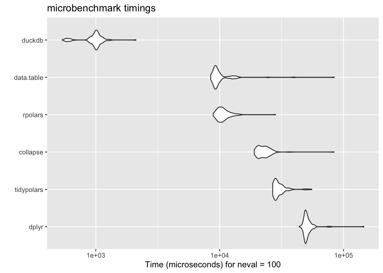
ggplot2::autoplot(res, order = "median")

expr	min	lq	mean	median	uq	max	neval
duckdb	535.255	930.782	975.5552	1003.270	1041.359	2109.532	100
data.table	8466.336	9103.620	11070.6416	9391.296	10083.130	83655.990	100
rpolars	8865.922	9778.111	10859.3018	10492.700	11356.447	28230.509	100
collapse	19025.927	20617.239	23333.6588	22573.144	24203.141	83712.775	100
tidypolars	26773.164	27874.383	30603.9724	28917.894	31457.804	55405.227	100
dplyr	43889.680	48724.380	52037.4189	50061.041	52284.840	145506.581	100

It is quite impressive how duckplyr is an order of magnitude faster than every other library. data.table and rpolars are the next fastest. Notably, there seems to be some overhead for the tidypolars package which loses some of the speed of rpolars. One has to note here though that both polars based packages are still under heavy development. Also, as the author Etienne points out in the comments, the overhead is constant so as soon as you work with really large data, you will not notice the difference as much anymore.

Join

The task for the join test os also quite straightforward. Calculate the average number of goals at home and away per team and join the resulting tables. For this task, we need to create individual join functions.

join_dplyr <- function(df) {
  home <- df |>
    summarise(mgh = mean(gh), .by = home) |>
    rename(team = home)
  away <- df |>
    summarise(mga = mean(ga), .by = away) |>
    rename(team = away)
  full_join(home, away, by = "team")
}

join_duck <- join_tpl <- join_dplyr

join_dt <- function(df) {
  home <- df[, .(mgh = mean(gh)), by = .(home)]
  away <- df[, .(mga = mean(ga)), by = .(away)]
  setnames(home, "home", "team")
  setnames(away, "away", "team")
  setkey(home, team)
  setkey(away, team)
  home[away, on = .(team), all = TRUE]
}

join_pl <- function(df) {
  home <- data_pl$group_by("home")$agg(pl$col("gh")$mean()$alias("mgh"))
  away <- data_pl$group_by("away")$agg(pl$col("ga")$mean()$alias("mga"))
  home <- home$rename("home" = "team")
  away <- away$rename("away" = "team")
  home$join(away, on = "team", how = "full")
}

join_collapse <- function(df) {
  home <- df |>
    fgroup_by(home) |>
    fsummarise(mgh = mean(gh)) |>
    frename(team = home)
  away <- df |>
    fgroup_by(away) |>
    fsummarise(mga = mean(ga)) |>
    frename(team = away)
  join(home, away, on = "team", how = "full", verbose = 0)
}

Here you see the advantage of tidypolars and duckplyr. Both can simply reuse the dplyr function and the packages do the magic in the background.

res <- microbenchmark::microbenchmark(
  times = 100,
  dplyr = join_dplyr(data_tbl),
  duckplyr = join_dplyr(data_duck),
  tidypolars = join_tpl(data_pl),
  data.table = join_dt(data_dt),
  rpolars = join_pl(data_pl),
  collapse = join_collapse(data_tbl)
)

ggplot2::autoplot(res, order = "median")

expr	min	lq	mean	median	uq	max	neval
duckplyr	3.694387	4.606924	5.091219	4.880948	5.191584	11.76397	100
rpolars	21.584614	23.764973	25.537319	25.761243	26.898419	31.67016	100
data.table	21.965463	23.529018	29.923670	29.180827	35.637979	60.86544	100
collapse	39.202191	42.658758	48.035470	44.975975	46.738565	148.10971	100
tidypolars	57.399139	61.233336	65.124748	64.182056	68.485395	94.56215	100
dplyr	134.835511	143.749116	150.810569	148.957776	152.985637	254.70332	100

The results remain pretty much the same as before. duckplyr is much faster than the remaining libraries, with rpolars and data.table on a similar level as the second best options.

Summary

As I said in the beginning, this was not a very comprehensive benchmark, but tailored to my personal use case scenarios. I would be really interested in more rigorous benchmarks but till then, I will happily switch to duckplyr for my backend.